Ramping constraints

Ramping constraints#

Ramping constraints are used to limit how much a variable, such as plant discharge and reservoir volume, can change over time in the optimization. Ramping constraints can be enforced by regulators for environmental reasons, such as limiting how fast the reservoir water level can change to protect wildlife living in the reservoir. They can also be technical in nature, and used to limit rapid changes in old machinery. This tutorial describes the different types of ramping that can be modelled in SHOP.

Standard ramping functionality#

The standard ramping functionality in SHOP enables the user to set an upper limit on the change of a variable between two consecutive time steps. Different limits can be set for maximum up-ramping (increase in variable value between two time steps) and maximum down-ramping (decrease in variable value between two time steps). In addition, a penalty cost may be given for breaking the ramping constraint. The table below gives an overview of the variable types that can have ramping restrictions. Searching for “ramp” or “ramping” in the attribute table on the SHOP Portal will give the complete list of ramping related attributes.

Object type	Variable	Direction	Ramping attribute	Unit	Global penalty	Object penalty
reservoir	volume	up	volume_ramping_up	Mm $^{3}$ /h	volume_ramp_penalty_cost
reservoir	volume	down	volume_ramping_down	Mm $^{3}$ /h	volume_ramp_penalty_cost
reservoir	level	up	level_ramping_up	m/h	level_ramp_penalty_cost
reservoir	level	down	level_ramping_down	m/h	level_ramp_penalty_cost
reservoir	volume	up	volume_amplitude_ramping_limit_up	Mm $^{3}$	volume_ramp_penalty_cost
reservoir	volume	down	volume_amplitude_ramping_limit_down	Mm $^{3}$	volume_ramp_penalty_cost
reservoir	volume	up	volume_nonseq_ramping_limit_up	Mm $^{3}$	volume_ramp_penalty_cost
reservoir	volume	down	volume_nonseq_ramping_limit_down	Mm $^{3}$	volume_ramp_penalty_cost
reservoir	level	up	level_amplitude_ramping_limit_up	m	level_ramp_penalty_cost
reservoir	level	down	level_amplitude_ramping_limit_down	m	level_ramp_penalty_cost
reservoir	level	up	level_nonseq_ramping_limit_up	m	level_ramp_penalty_cost
reservoir	level	down	level_nonseq_ramping_limit_down	m	level_ramp_penalty_cost
plant	production	up	power_ramping_up	MW/h	production_ramp_penalty_cost
plant	production	down	power_ramping_down	MW/h	production_ramp_penalty_cost
plant	discharge	up	discharge_ramping_up	m3s/h	production_ramp_penalty_cost
plant	discharge	down	discharge_ramping_down	m3s/h	production_ramp_penalty_cost
gate	discharge	up	ramping_up	m3s/h	gate_ramp_penalty_cost	ramp_penalty_cost
gate	discharge	down	ramping_down	m3s/h	gate_ramp_penalty_cost	ramp_penalty_cost
river	flow	up	ramping_up	m3s/h	gate_ramp_penalty_cost	ramping_up_penalty
river	flow	down	ramping_down	m3s/h	gate_ramp_penalty_cost	ramping_down_penalty
contract	outtake	up	ramping_up	MW/h		ramping_penalty_cost_up
contract	outtake	down	ramping_down	MW/h		ramping_penalty_cost_down

As seen from the units, max ramping is specified per hour. If the time step length is different than one hour, the max ramping value will be scaled accordingly by the model.

Amplitude and non-sequential ramping functionality#

Ramping on reservoir volume has two special types of ramping constraints that are provided in the SHOP_NONSEQ_AMPLITUDE_RSV_RAMP license. These constraints are given as xyt. Example of use is given in this example.

Non-sequential volume ramping#

Non-sequential ramping on reservoir volume adds ramping constraints between two non-sequential time steps, such as ramping between the first hour of day one and the first hour of day two. The input is given as an xyt. Datastructure specification is given under the respective attributes: volume_nonseq_ramping_limit_up, volume_nonseq_ramping_limit_down, level_nonseq_ramping_limit_up, level_nonseq_ramping_limit_down.

Amplitude volume ramping#

Amplitude ramping on reservoir volume is similar to non-sequential ramping, but adds ramping constraints from the first specified time step to all time steps within the same ramping period. Datastructure specification is given under the respective attributes: volume_amplitude_ramping_limit_up, volume_amplitude_ramping_limit_down, level_amplitude_ramping_limit_up, level_amplitude_ramping_limit_down.

Old ASCII format#

These attributes have previously been defined in ASCII using a special TTXY format, which will be supported in a transition period. However, we strongly recommend changing to the new format.

Complex ramping functionality#

It is possible to specify more advanced ramping constraints for reservoir level and plant discharge. The complex ramping functionality, which requires the SHOP_COMPLEX_RAMPING license, implements two new ramping types: rolling ramping and period ramping. These concepts are described in more detail below, and the two examples for complex plant ramping and complex reservoir ramping shows how to use all different complex ramping constraints in practice.

Rolling ramping constraints#

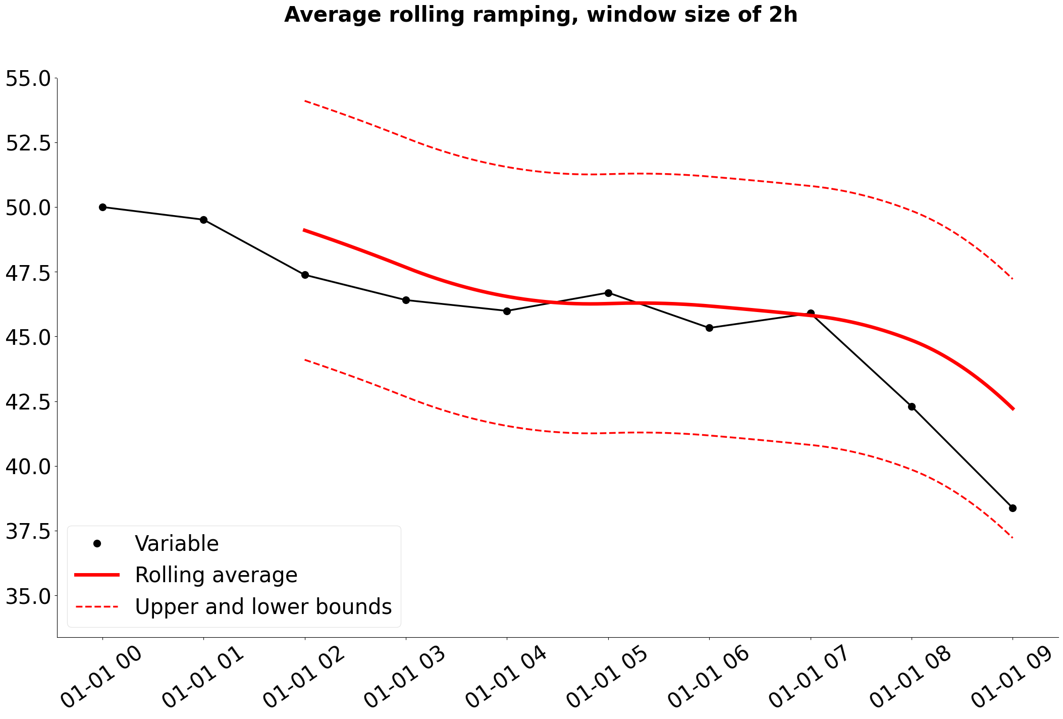
Rolling ramping constraints limit the reservoir level or plant discharge based on the previous values in a rolling time window with a specified length. The ramping limit can either be specified to be a maximal deviation upward or downward from the average in the rolling window, or as the maximal deviation upward/downward from the maximal/minimal value in the rolling window. These sub-types of rolling ramping constraints are called average rolling ramping and limit rolling ramping.

Figure 1 and 2 illustrate how average rolling ramping and limit rolling ramping are applied to a generic variable that changes linearly between optimized values, such as the reservoir level.


Figure 1: Rolling average ramping bounds are calculated in either direction around the rolling average value.


Figure 2: The upper bound for rolling limit ramping is calculated upwards from the rolling minimum value, while the lower bound is calculated downwards from the rolling maximum value.

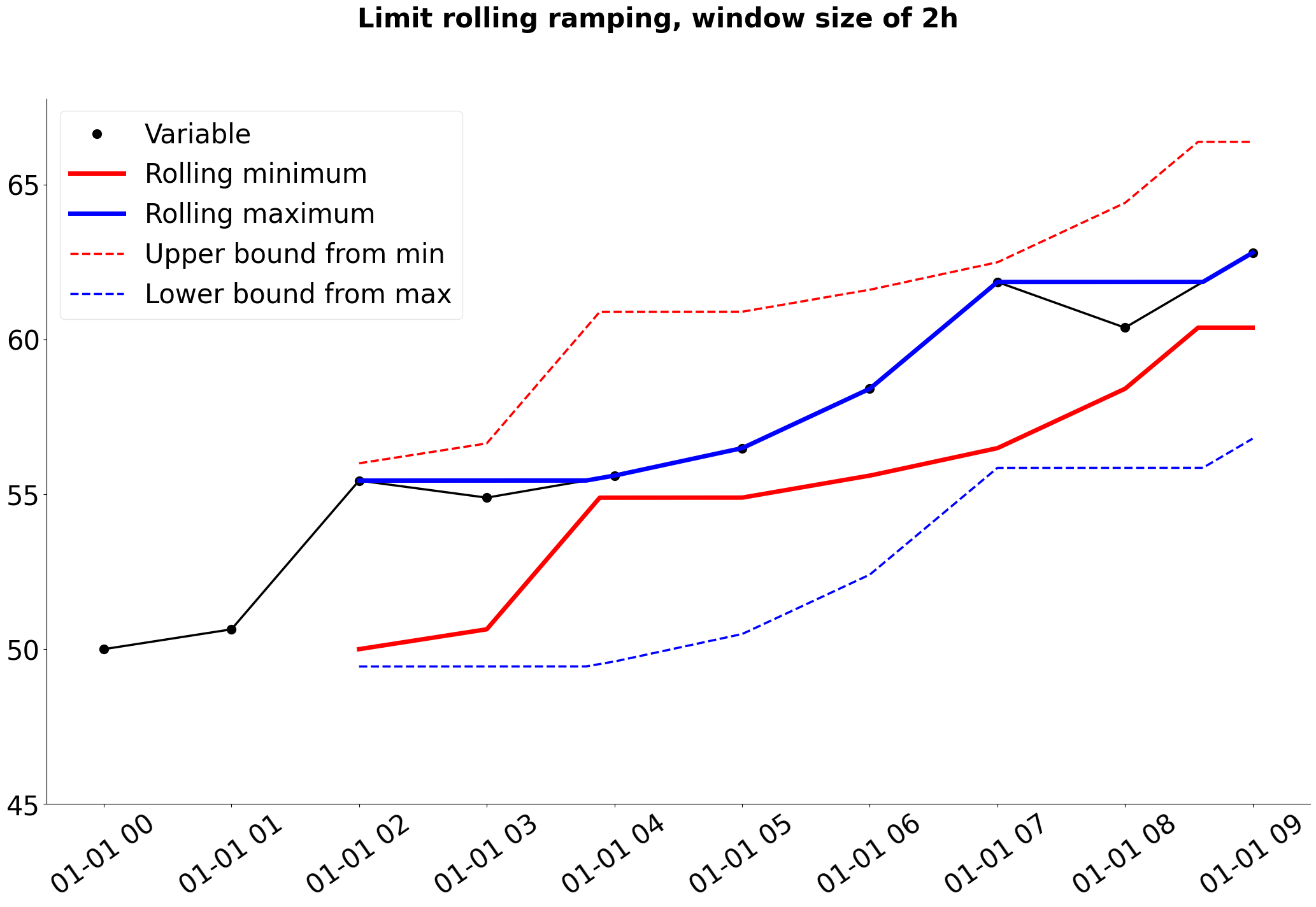
Note that the rolling average in Figure 1 and the rolling minimum and maximum values in Figure 2 are shown as continuous functions in time. However, optimization models such as SHOP discretize the time dimension and only have one variable per time step. This means that the rolling average, minimum, or maximum values are only calculated at the beginning of each time step in SHOP, not continuously.

There are a total of four rolling ramping constraint attributes on the reservoir object: average_level_rolling_ramping_up and down, and limit_level_rolling_ramping_up and down. Similar attributes are found on the plant object related to discharge instead: average_discharge_rolling_ramping_up and down, and limit_discharge_rolling_ramping_up and down. These input attributes are of the type XYT, which makes it possible to specify multiple ramping constraints with different window sizes to the same object. It also makes it possible to change the ramping limit (or deactivate the constraint) inside the optimization interval. The XYT datatype consists of several XY tables each referred to a timestamp. The timestamp specifies from when the data in the XY table is valid. The XY table is valid from the specified time and onwards until the time of the next XY table with a later time stamp is reached. The x-values in the XY tables specify the window size in minutes of the rolling ramping constraint in question, while the y-values specify the ramping limit in meters. This makes it possible to give in multiple ramping constraint of the same type on the same object but with different window sizes. To deactivate a ramping constraint, a NaN value may be passed as a y-value instead of the ramping limit. Usage of multiple constraints with different window sizes is shown in this reservoir level example, while changing or deactivating complex ramping constraints is shown in this plant discharge example.

Penalty costs for violating the different rolling ramping constraints can be specified with the TXY attribute level_rolling_ramping_penalty_cost on the reservoir object and discharge_rolling_ramping_penalty_cost on the plant object. Otherwise, the global level_ramp_penalty_cost and plant_discharge_ramp_penalty_cost found on the global_settings object are used instead.

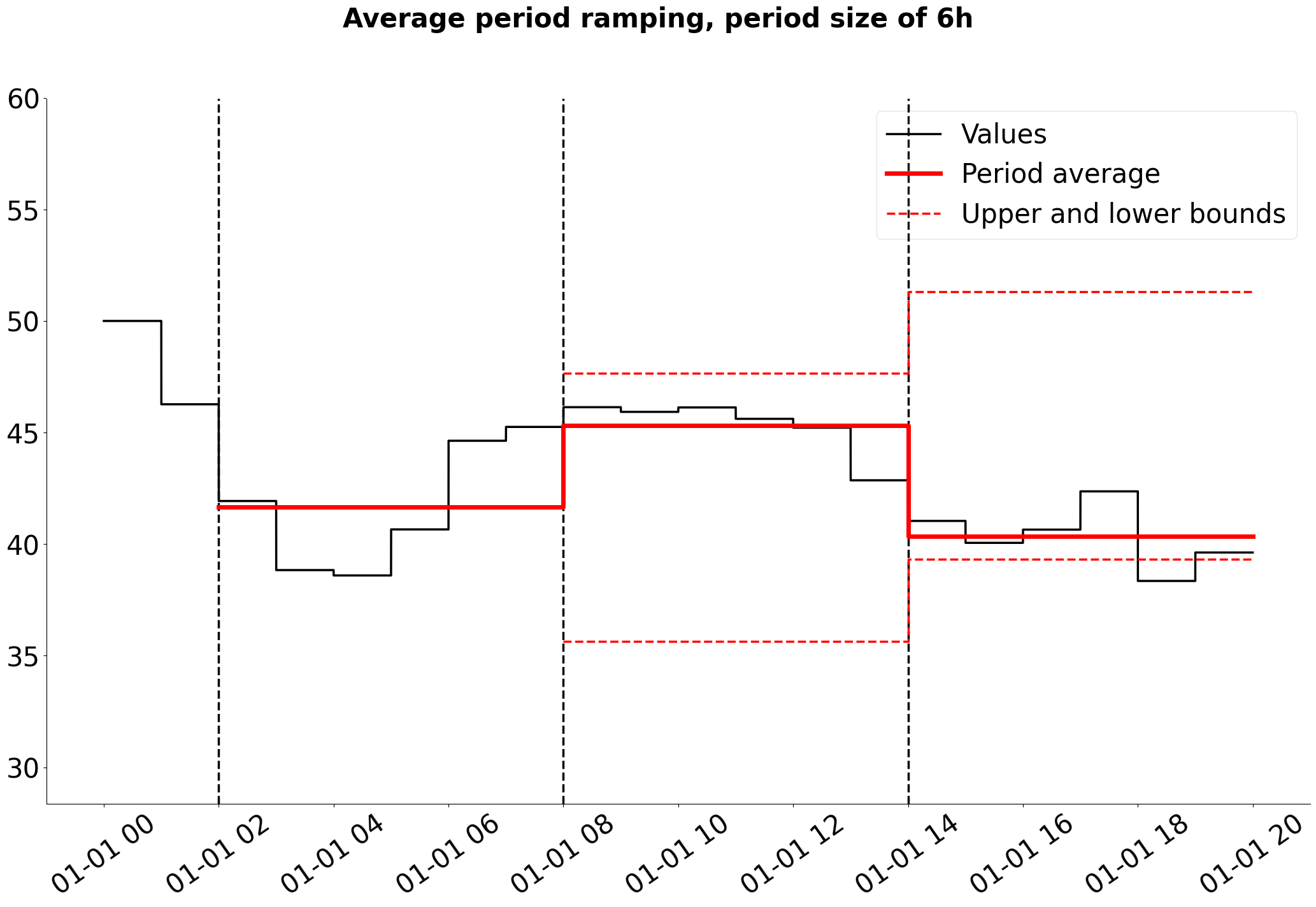
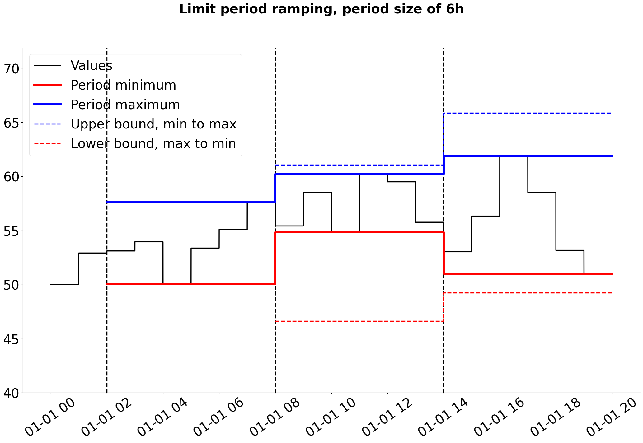
Period ramping constraints#

Period ramping is fundamentally different from the rolling ramping constraints as they are related to fixed time periods instead of a rolling time window. The period ramping constraints are also not applied to the reservoir level or plant discharge for every time step, instead they limit the change of the average, minimum or maximum values from one period to the next. Average period ramping will therefore limit the change in the average value from one period to the next. Similarly, limit period ramping constrains the maximum (minimum) value in one period based on the minimum (maximum) value in the preceding one. Period ramping is usually used to model ramping constraints that are related to calendar time, such as limiting the change in the average plant discharge from one day to the next.

Figures 3 and 4 illustrate the different period ramping constraints for a generic variable that is constant over a time interval, such as plant discharge.


Figure 3: Upper and lower bounds for the average value within each fixed time period are calculated based on the average value in the preceding period. The start of each fixed time period is shown as vertical dashed lines. Note that individual values may be outside the ramping bounds since it is the average period value that is constrained.


Figure 4: The upper bound for the maximal period value is calculated based on the minimal value in the previous period, and the lower bound for the minimal period value is calculated based on the maximal value in the previous period. The start of each fixed time period is shown as vertical dashed lines.

There are a total of four period ramping constraint attributes on the reservoir object: average_level_period_ramping_up and down, and limit_level_period_ramping_up and down. Similar attributes are found on the plant object related to discharge instead: average_discharge_period_ramping_up and down, and limit_discharge_period_ramping_up and down. As discussed in the section on rolling ramping constraints, the input attributes for period ramping are also XYTs and have analogous interpretations.

Penalty costs for violating the different period ramping constraints can be specified with the TXY attribute level_period_ramping_penalty_cost on the reservoir object and discharge_period_ramping_penalty_cost on the plant object. Otherwise, the global level_ramp_penalty_cost and plant_discharge_ramp_penalty_cost found on the global_settings object are used instead.

In addition to the XYT attributes to define the ramping constraints themselves, additional SY attributes can be supplied to specify the start time of the first fixed period. These are called average_level_period_ramping_up_offset and so on, one for each period ramping XYT input attribute. The y-values in the offset attributes must match the x-values (ramping period size in minutes) of the corresponding XYT attribute, while the string values are time stamps that specify the start time of the first full ramping period. The offset time stamp is internally converted by SHOP to a whole number of minutes relative to the start time of the optimization. In Figure 3 and 4, the first period starts 2 hours after optimization start, which indicates that an offset of 120 minutes has been used.

It is common to end up with fractional ramping periods in the optimization. This happens when the length of the optimization horizon is not a whole number of ramping periods, and/or when an offset is specified for the start of the first ramping period. If no offset is specified, the first ramping period starts at the beginning of the optimization horizon and any fractional ramping period will be left at the end of the horizon. If the last ramping period in the optimization is fractional, no ramping constraints will be built for that period. There is no fractional ramping period at the end of the horizon in Figures 3 and 4, but the first whole ramping period starts 2 hours after the beginning of the optimization. The initial two hour long fractional period can be completed by giving in historical values to SHOP, which is explained in the next section.

Historical values#

Since both rolling and period ramping constraints look backwards in time when calculating the ramping boundaries, it is necessary to specify historical level and discharge values to create ramping constraints for the fist hours of the optimization. This is given to SHOP in the form of two TXY attributes called historical_level and historical_discharge. These attributes are regular TXYs, but should start before the start time of the optimization. Any values in the historical TXYs that are inside the optimization horizon are ignored.

For rolling ramping constraints, it is sufficient to include historical values as far back as the longest rolling window length before the start time of the optimization. The examples of rolling ramping shown in Figures 1 and 2 have a rolling window length of 2 hours, and so historical values that cover at least 2 hours before the optimization starts are needed. This is also why the rolling average, minimum, and maximum values are not plotted for the first two hours in the figures.

For period ramping, it is sufficient to have enough historical data to completely fill any fractional period at the start of the optimization in addition to one purely historical period before that. The values in the purely historical period is used to calculate bounds for the first (potentially fractional) ramping period in the optimization. In the example shown in Figures 3 and 4, the period length is 6 hours and the offset of the first whole period is 2 hours. This means that a total of 10 historical hours are needed: 4 hours to complete the fractional period and then 6 hours to have a purely historical period to calculate the initial ramping bounds for the (now complete) initial ramping period.

Note that there are no limitations to giving in more historical data than is strictly needed. The data that is older than the relevant historical period is simply ignored.