PQ curves#
This documentation gives an introduction to PQ curves in SHOP. A more detailed description can be found in this paper.
The hydropower production function converts the kinetic energy of falling water into electrical energy as it flows through the turbine of a generator, and it is the fundamental equation of SHOP. It is a complex, non-linear equation with state dependency, given by
where \(p_{i,s,t}\) is the production for unit \(i\) at plant \(s\) at time step \(t\), \(\textup{G}\) is a conversion constant including the gravity acceleration and water density, \(\eta_{i,s}^{\textup{GEN}}\) is the generator efficiency, \(\eta_{i,s}^{\textup{TURB}}\) is the turbine efficiency, \(h_{i,s,t}^{\textup{EFF}}\) is the effective generator head, and \(q_{i,s,t}\) is the discharge. Note that \(\eta_{i,s}^{\textup{GEN}}\) depends on the generated power, which makes the equation implicit in terms of \(p_{i,s,t}\). The turbine efficiency depends on both the discharge through the turbine and the effective generator head, both of which are variables in SHOP. Successive refinement of the linearization of the PQ relationship is used in SHOP to tackle these non-linearities.
Mechanical efficiency#
SHOP uses information from the generator attributes gen_eff_curve and turb_eff_curves to build the PQ curves. The turb_eff_curves give the turbine efficiency \(\eta^{\textup{TURB}}\) as a function of \(q\) for different values of the effective head \(h^{\textup{EFF}}\), as illustrated in the figure below. Each curve is a slice of the hill chart of the turbine where the head is constant.
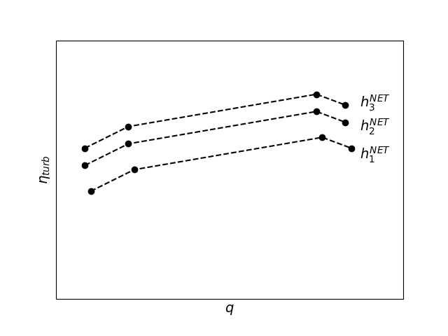
The generator efficiency is assumed to only depend on the generated power of the generator, and so only requires a single input curve with the efficiency for different power production levels.
Effective head and head loss#
The effective generator head is the gross head of the power plant minus any head loss incurred from above or below the plant. The effective head depends on the discharge of all units in the plant since there are many shared head losses, such as the loss in the shared main tunnel and the loss in shared penstocks. Head losses defined by a single coefficient, such as main_loss and penstock_loss on a plant, are assumed to be quadratic in the discharge \(q\):
It is also possible to specify intake_loss and tailrace_loss tables on a plant which describes additional head loss directly as a piece-wise linear function of the total plant discharge. The total head loss for a unit is the sum of the head loss in all the individual components. The eff_head attribute on the generator saves the effective head for each time step in the optimization, while gross_head is reported on the plant object. The unit head_loss is also reported.
Initial PQ curves#
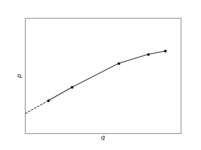
The original_pq_curves attribute refer to the relationship between production and discharge including all operating limits before any polishing is applied.
The first step is to find the minimum and maximum discharge points, \(Q^{\textup{MIN}}_{i,s,t}\) and \(Q^{\textup{MAX}}_{i,s,t}\), as well as the best efficiency point \(Q^{\textup{BEST}}_{i,s,t}\). If these are independent on the plant effective head \(h^{\textup{EFF}}\), they can be used directly. Otherwise, \(h^{\textup{EFF}}\) must first be determined. The water levels obtained in the previous iteration in SHOP is used to estimate the plant’s gross head \(h^{\textup{GROSS}}\). Assuming that \(h^{\textup{EFF}}_{i,s,t}=h^{\textup{GROSS}}_{i,s,t}\) as a starting point, \(h^{\textup{EFF}}\) can then be determined by an iterative process using the information from the turb_eff_curves and interpolation. This process is more accurate in incremental iterations where the unit commitment decisions have been fixed, since this makes the error in the head loss calculation is lower.
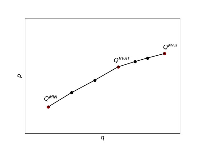
After \(Q^{\textup{MIN}}_{i,s,t}\), \(Q^{\textup{BEST}}_{i,s,t}\) and \(Q^{\textup{MAX}}_{i,s,t}\) have been found, the intervals between \(Q^{\textup{MIN}}_{i,s,t}\) and \(Q^{\textup{BEST}}_{i,s,t}\) and \(Q^{\textup{BEST}}_{i,s,t}\) and \(Q^{\textup{MAX}}_{i,s,t}\) are uniformly partitioned. The number of points below \(Q^{\textup{BEST}}_{i,s,t}\) can be set using the global setting n_seg_down, or the plant attributes n_seg_down (in incremental mode) and n_mip_seg_down (in full mode). Likewise, the number of points above \(Q^{\textup{BEST}}_{i,s,t}\) can be set using the global setting n_seg_up, or the plant attributes n_seg_up (in incremental mode) and n_mip_seg_up (in full mode). To improve convergence, the optimized discharge \(q_{i,s,t}\) from the previous iteration is used as an extra breakpoint. The corresponding power output is then found for each breakpoint by solving the hydropower production function.
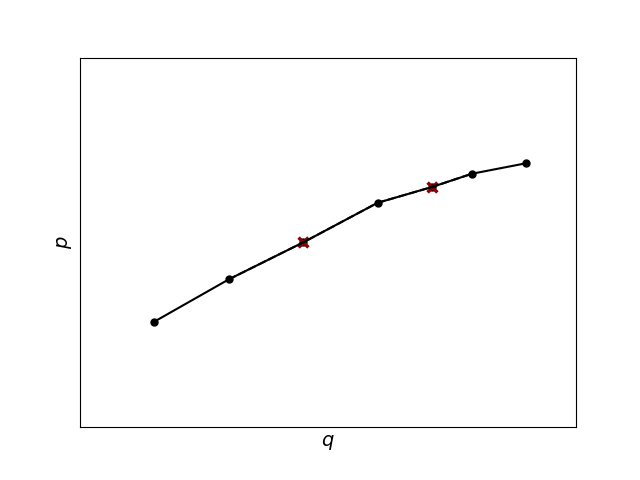
Convexification and incorrect uploading#
The convex_pq_curves attribute refers to the PQ curves after convexification. The slope of each segment of the PQ curve is made non-increasing by removing the non-concave breakpoints as illustrated in the figure below. This is done to encourage the PQ curve to be uploaded correctly in the optimization without introducing extra binary variables for each segment. As long as the slope of each segment is non-decreasing, the optimization problem will usually use segment 1 before segment 2 and so on since this minimizes the water use. It is still possible to get an incorrect uploading of the PQ curves in SHOP, this usually happens if there is some incentive to use more water than necessary to produce power. If it is necessary to move a lot of water through the system, perhaps due to high inflow and the risk of spillage, incorrect uploading can become a problem if strict production constraints are applied to the power plant with max_p_constr. Any other incentive to waste water (inconsistent water values, negative prices in combination with forced operation) could also lead to incorrect uploading of the segments in the PQ curve. There is no guarantee that the PQ curve will be uploaded correctly without using binary variables (which would increase calculation time) or using only a single segment (which would be inaccurate). The command set simple_pq_recovery /on will do the latter and build a PQ curve with only a single segment up to \(Q^{\textup{MAX}}\), but only for time steps and plants where incorrect uploading has been detected in a previous iteration.
Final operating limits#
The final operating limits are found based on the most restrictive rule. Limits can come from the plant attributes min_p_constr, max_p_constr, min_q_constr and max_q_constr, or from the generator attributes p_min, p_max, min_p_constr, max_p_constr, min_q_constr and max_q_constr. If the limit comes from production, the corresponding \(q\) is calculated.
The minimum and maximum discharge limits for the PQ curves are found from the turb_eff_curves by default. It is also possible to set these limits independently as a function of effective head by using the generator attributes min_discharge and max_discharge. This is described in more detail in the PQ curve limits example.
The final_pq_curves attribute refers to the curves that are directly included in the optimization problem formulated by SHOP. If mip_flag is on, the first point of the PQ curves are extended to \(q=0\) in full iterations. If mip_flag is off in full iterations, the PQ curves will be extended to include \((p,q)=(0,0)\) from the best efficiency point. This is to ensure correct calculations from the best efficiency point and upwards, and to avoid negative production for zero discharge.