

Power flow#
SHOP implements PTDF-based power flow. The busbar and ac_line objects are used to specify the grid topology of the model. The following example demonstrates a simple model with power flow and thermal production units.
Set up model#
First, we initialize the model
import pandas as pd
import plotly.graph_objs as go
from pyshop import ShopSession

shop = ShopSession()
starttime=pd.Timestamp("2022-02-27T00")
endtime=starttime+pd.DateOffset(hours=24)
shop.set_time_resolution(starttime=starttime, endtime=endtime, timeunit="hour")
Add busbars and set the load. The load in busbar 1 is linearly increasing over time in this example, while all other input data is constant.
b1=shop.model.busbar.add_object("Busbar1")
b1.load.set(pd.Series([50+i for i in range(24)],index=[starttime+pd.Timedelta(hours=i) for i in range(24)]))
b2=shop.model.busbar.add_object("Busbar2")
b2.load.set(60)
b3=shop.model.busbar.add_object("Busbar3")
b3.load.set(300)
Then we define one thermal unit for each busbar and connect them. The marginal cost of the thermal units is equal to the fuel_cost in this case since n_segments is set to 1. Busbar 3 has the largest thermal unit, while busbar 1 has the cheapest one. Only a small and expensive unit is located in busbar 2.
t1=shop.model.thermal.add_object("Thermal1")
t1.fuel_cost.set(75)
t1.n_segments.set(1)
t1.min_prod.set(0)
t1.max_prod.set(140)
t1.connect_to(b1)

t2=shop.model.thermal.add_object("Thermal2")
t2.fuel_cost.set(180)
t2.n_segments.set(1)
t2.min_prod.set(0)
t2.max_prod.set(20)
t2.connect_to(b2)

t3=shop.model.thermal.add_object("Thermal3")
t3.fuel_cost.set(140)
t3.n_segments.set(1)
t3.min_prod.set(0)
t3.max_prod.set(400)
t3.connect_to(b3)
There are three AC lines that connect the busbars, and there is no power loss in the transmission. The AC line connecting busbar 2 and 3 has the lowest transmission capacity, which is specified in both directions by the max_forward_flow and max_backward_flow attributes. Note that the positive (forward) flow direction on each line is determined by the connections between the busbar and ac_line objects.
Create AC lines and connect between buses:
ac1=shop.model.ac_line.add_object("AC_line1")
ac1.max_forward_flow.set(40)
ac1.max_backward_flow.set(40)
b1.connect_to(ac1)
ac1.connect_to(b2)

ac2=shop.model.ac_line.add_object("AC_line2")
ac2.max_forward_flow.set(250)
ac2.max_backward_flow.set(250)
b1.connect_to(ac2)
ac2.connect_to(b3)

ac3=shop.model.ac_line.add_object("AC_line3")
ac3.max_forward_flow.set(10)
ac3.max_backward_flow.set(10)
b2.connect_to(ac3)
ac3.connect_to(b3)
The we set the PTDF matrix that determines the flow on each line as a function of the net power injection in each busbar. Busbar 3 is chosen as the slack bus in this example, which means that the PTDF values for busbar 3 are all zero.
ac_lines=["AC_line1", "AC_line2", "AC_line3"]
b1.ptdf.set(pd.Series(data=[0.2/0.5, (0.2+0.1)/0.5, 0.2/0.5], index=ac_lines))
b2.ptdf.set(pd.Series(data=[-0.1/0.5, 0.1/0.5, (0.2+0.2)/0.5], index=ac_lines))
b3.ptdf.set(pd.Series(data=[0.0, 0.0, 0.0], index=ac_lines))
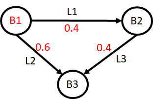
The grid topology with the PTDFs visualized for busbars 1 and 2 are shown in the figures below.
|
|---|
Grid topology with the PTDF for busbar 1 shown as red numbers. |
|
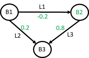
|---|
Grid topology with the PTDF for busbar 2 shown as green numbers. Note that the PTDF for line 2 is negative due to the chosen positive line direction. |
Run the model:
shop.start_sim([],["1"])
Results#
First, we take a look at the production of each unit in the system. The cheapest unit located in busbar 2 does not operate at full capacity until 15 hours after optimization start, this is due to the transmission line constraints and PTDF values used in the example.
p1 = t1.production.get()
p2 = t2.production.get()
p3 = t3.production.get()

fig = go.Figure()
fig.add_trace(go.Scatter(x=p1.index, y=p1.values, name="Sum production busbar 1"))
fig.add_trace(go.Scatter(x=p2.index, y=p2.values, name="Sum production busbar 2"))
fig.add_trace(go.Scatter(x=p3.index, y=p3.values, name="Sum production busbar 3"))
fig.update_layout(xaxis_title="Time", yaxis_title="Production [MW]")
fig.show()
The total net power injection in each busbar determines the flow on each line in combination with the PTDF matrix.
l1 = b1.load.get()
l2 = b2.load.get()
l3 = b3.load.get()

fig = go.Figure()
fig.add_trace(go.Scatter(x=l1.index, y=p1.values-l1.values, name="Net injection busbar 1"))
fig.add_trace(go.Scatter(x=l2.index, y=p2.values-l2.values, name="Net injection busbar 2"))
fig.add_trace(go.Scatter(x=l3.index, y=p3.values-l3.values, name="Net injection busbar 3"))
fig.update_layout(xaxis_title="Time", yaxis_title="Power [MW]")
fig.show()
The resulting flow on each power line is shown below. Note that the line between busbar 2 and 3 operates at full (reverse) capacity for all times.
flow_12 = ac1.flow.get()
flow_13 = ac2.flow.get()
flow_23 = ac3.flow.get()

fig = go.Figure()
fig.add_trace(go.Scatter(x=flow_12.index, y=flow_12.values, name="Flow from 1 to 2"))
fig.add_trace(go.Scatter(x=flow_13.index, y=flow_13.values, name="Flow from 1 to 3"))
fig.add_trace(go.Scatter(x=flow_23.index, y=flow_23.values, name="Flow from 2 to 3"))
fig.update_layout(xaxis_title="Time", yaxis_title="Power flow [MW]")
fig.show()
Finally, we can plot the dual value of the power balance in each busbar by retrieving the energy_price attribute, which represents the nodal price. Busbars 2 and 3 have a constant price equal to the marginal cost of their respective thermal units. This is also true for busbar 1 initially when its thermal unit operates below maximum capacity. From hour 15, the price in busbar 1 jumps up to 160 €/MWh, which is the average of the price in the other busbars. This is caused by the constrained line between busbar 2 and 3, which forces the increasing load in busbar 1 to be served by increasing the production of both the thermal unit in busbar 2 and 3 by the same amount. The marginal cost of increasing the load in busbar 1 is therefore 50% of the marginal cost of unit 2 plus 50% of the marginal cost of unit 3.
price_1 = b1.energy_price.get()
price_2 = b2.energy_price.get()
price_3 = b3.energy_price.get()

fig = go.Figure()
fig.add_trace(go.Scatter(x=price_1.index, y=price_1.values, name="Price in busbar 1"))
fig.add_trace(go.Scatter(x=price_2.index, y=price_2.values, name="Price in busbar 2"))
fig.add_trace(go.Scatter(x=price_3.index, y=price_3.values, name="Price in busbar 3"))
fig.update_layout(xaxis_title="Time", yaxis_title="Power price [€/MWh]")
fig.show()